This page aims to give an overview of DGrowthR and
introduce you to the main functions that you might want to use for your
own analysis. Broadly speaking, this tutorial is divided into the
following sections:
-
Preparing your data for
DGrowthR. [Required] - Preparing a DGrowthR object. [Required]
- Pre-processing. [Required]
- Exploratory data analysis.
- Growth parameter calculation.
- Differential growth testing.
- Multiple differential growth testing.
library("DGrowthR")
library("tidyverse")

# We also need the permApprox package for the permutation test in the growth comparison section
# Here we install if it wasn't already installed
if(!requireNamespace("permApprox", quietly = TRUE)) {
  remotes::install_github("stefpeschel/permApprox")
}
Preparing your data for DGrowthR.
To start our analysis we first need to prepare a
DGrowthR::DGrowthR() object. To do this, we require two
sources of information:
1. Growth data. 2. Metadata.
Below we will go into more details of each one.
Growth data.
DGrowthR can be used to analyse growth data from
multi-well plate readers. Depending on the specific platform that is
used, the actual output of each machine might look slightly different.
DGrowthR assumes your data consists of simultaneous
measurements of growth, preferably that are regularly
interspaced. This means that the growth across all wells is measured at
the same time and, ideally, that the time between measurements is always
the same. If the data is not measured at regular intervals,
DGrowthR will still be able to analyze your data. Examples
of the kinds of data the can be used can be seen in our Source
Data folder.
** Below is an example of the data collected for one 384 well plate
from Brenzinger
2024. This dataframe could be used directly to build a
DGrowthR::DGrowthR() object. The important features
include: **
- A column called Time: The values in this column
indicate the time at which the OD measurements were made for all of the
wells in this plate. The units of the Time column
(seconds, minutes, hours) are taken as is. No unit conversion
is performed by
DGrowthR.
- Columns indicating wells: All of the columns besides the
Time column indicate the wells in the plate. The values
are the measured optical density in each well at a specific time
point.
- An arbitrary number of wells can be present (typically 384 or 96). Typically, each well is identified as a combination of an uppercase letter followed by a number, with no spaces. This information is used to identify each individual growth curve.
Source_Data/Brenzinger_2024/wt_1_OD.txt
# Read example data from Brenzinger 2024
example_brenzinger <- read.delim("../Source_Data/Brenzinger_2024/od_data/wt_1_OD.txt",
                                 sep = '\t')

tibble(example_brenzinger) %>%
  rmarkdown::paged_table()
As stated above, this data frame could be used directly by
DGrowthR.
What if I want to analyze data from multiple plates?.
This is definitely possible with DGrowthR. There are
just a couple of things to keep in mind:
The data for each plate should be in separate files.
It is assumed that measurements are taken at roughly the same timepoints across all plates. This means that the Time column should be roughly the same for all plates. Due to small variations between different plate measurements, the values in the Time column might be slightly different.
Each growth curve will now be identified as the combination of {plate name}_{well}.
In order to read the data from multiple plates, harmonize the
Time column, and assign individual curve identifiers in
a way that can be used by DGrowthR, we provide a standalone
function called read_multiple_plates(). Below, we use it to
read all of the data from the Brenzinger
2024 study. In this case we know that 20 measurements are taken; the
time between the first and second measurement is ~2 hours, followed by
regular 44 minute intervals. This can help us create a common time
vector for all files.
# Create common time vector
common_time_vector <- c(0, 2, seq(from=2.739, by=0.739, length.out=18))

# Read all OD data
brenzinger_data <- read_multiple_plates(path_target = "../Source_Data/Brenzinger_2024/od_data/",
                                        time_vector = common_time_vector)
#> The following OD data was found: dCBASS_1_OD.txt, dCBASS_2_OD.txt, dCBASS_3_OD.txt, wt_1_OD.txt, wt_2_OD.txt, wt_3_OD.txt
The output of this function is a list with two data frames. First is the “od_data” data frame. As you can see, it has a common Time column with each individual growth curve in remaining columns. Each growth is now identified with a curve_id which is built as {plate_name}_{well}, with the plate_name actually just being the name of the file from which the data was read, without the extension. In total there are 20 measurements for 2,304 (384 * 6) growth curves!
# Show the first five columns of the complete OD data
brenzinger_od <- brenzinger_data[["od_data"]]


brenzinger_od %>%
  rmarkdown::paged_table()
Additionally, a “metadata” data frame is provided. This data frame explains where each curve_id is coming from. The plate name (file name without the extension) and the original well are explicitly mentioned.
brenzinger_metadata <- brenzinger_data[["metadata"]]


brenzinger_metadata %>%
  rmarkdown::paged_table()
This sets us up nicely to now discuss the metadata.
Metadata.
The metadata contains all of the information relevant to the experimental setup. The information contained here can be quite arbitrary and suit the needs of the researcher. For example, it can contain information about the conditions under which each growth curve was measured, replicate number, batch number, etc. Importantly, there must be a column named curve_id, that contains the names of all of the growth curves present in the data frame with the optical density information.
In our case, we will use the information about genotype, compound and concentration provided by the original study.
# Information about each plate
database.df <- read_tsv("../Source_Data/Brenzinger_2024/Database.txt",
                        show_col_types = FALSE) %>%
  separate(Strain, into = c("genotype", NA)) %>%
  select(file_id, genotype, Rep_Nr) %>%
  mutate(plate_name = tools::file_path_sans_ext(file_id))

# Information about each well
mapper.df <- read_tsv("../Source_Data/Brenzinger_2024/Map.txt",
                       show_col_types = FALSE) %>%
  rename("well" = "Well")


# Add this information to the metadata data frame
brenzinger_metadata <- brenzinger_metadata %>%
  left_join(database.df, by="plate_name") %>%
  left_join(mapper.df, by="well") %>%
  unite("genotype_well", c(genotype, well), sep="_", remove=FALSE)

brenzinger_metadata %>%
  rmarkdown::paged_table()
Now we have a lot more information about the conditions under which
each growth curve was gathered. With these sources of information, we
can now build our DGrowthR::DGrowthR() object.
Building a DGrowth object.
Once we are satisfied with our growth data and metadata data frames,
we can instantiate a DgrowthR() object with the
DgrowthRFromData() function.
# Instantiate a DGrowthR object
dgobj <- DGrowthRFromData(od_data = brenzinger_od,
                          metadata = brenzinger_metadata)
#> Creating a DGrowthR object...
#> 2304 growth curves.
#> 20 timepoints.
#> 8 covariates (including well).
We now have a DGrowthR object. This is the heart of our package. All
functions require a DGrowthR object as input. For example,
we can quickly visually inspect our data using the
plot_growth_curves() function.
plot_growth_curves(dgobj)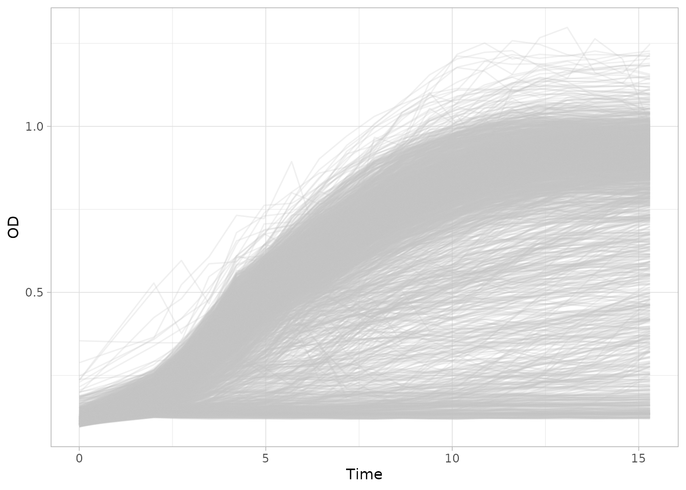
We can inspect our growth curves using variables of the metadata with
the facet and color parameters.
plot_growth_curves(dgobj, facet="plate_name", color="genotype")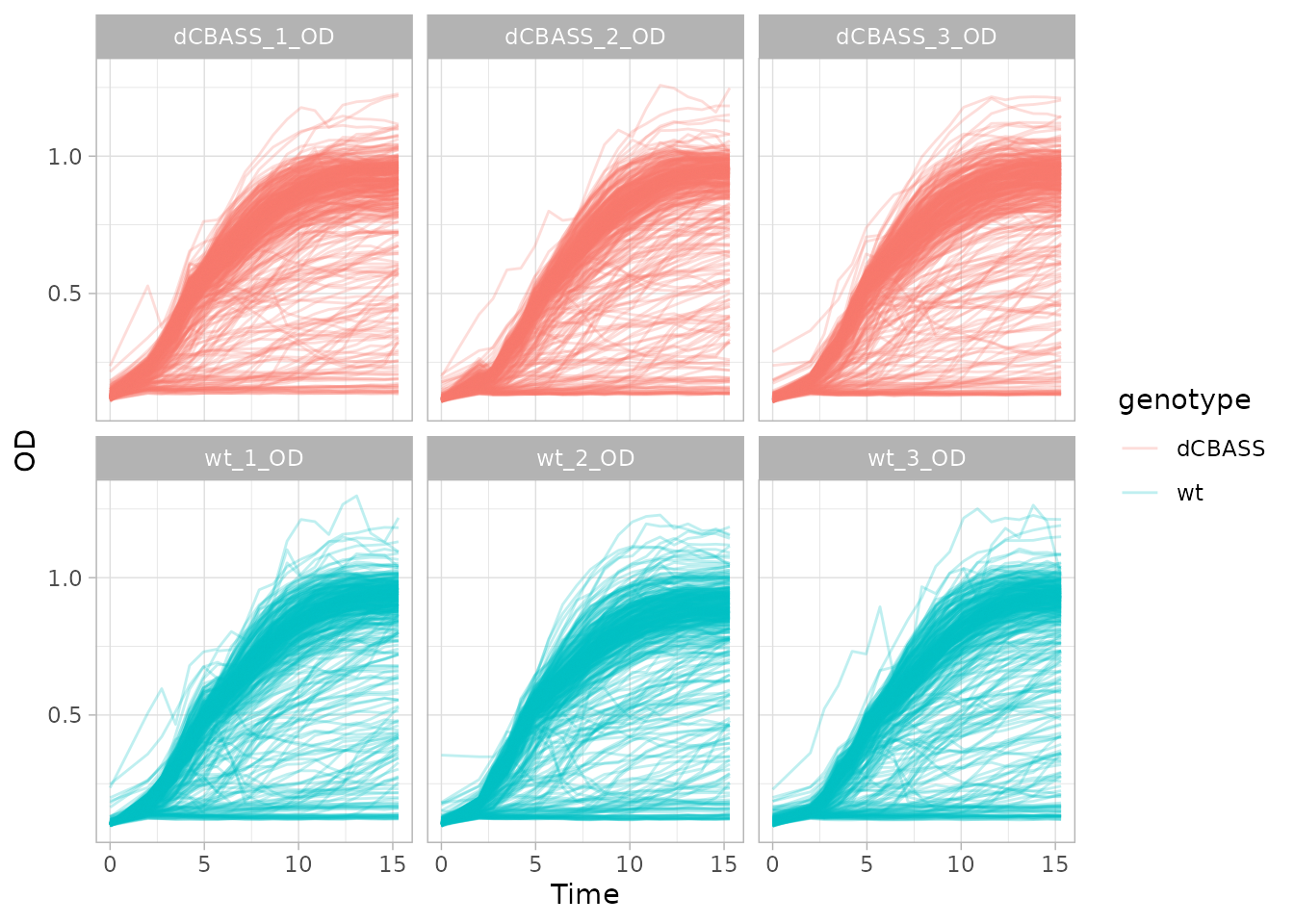
It’s worth mentioning that all of the plots returned by
DGrowthR functions are ggplot objects. Meaning you
may further customize them to your liking using ggplot syntax and
functions.
Now that our data is ready we can start pre-processing.
Pre-processing.
Pre-processing growth curves is essential before performing any
analysis. This is done by the preprocess_data() function.
The following transformations are performed:
First the user may specify if some of the initial growth measurements should be ignored with the
skip_first_n_timepointsparameter. All growth curves would be shortened so they start at timepoint skip_first_n_timepoints + 1.The optical density measurements are log-transformed. This enables accurate estimation of growth parameters such as maximum specific growth rate, end of lag phase, etc. Both the log and linear scaled data are conserved.
Baseline correction is performed by subtracting the initial OD measurement from the rest of the growth curve.
dgobj <- preprocess_data(dgobj)
#> Log-transforming the growth measurements...
#> Using OD from timepoint 1 as baseline.
We can see how our data has been transformed.
plot_growth_curves(dgobj, facet="plate_name", color="genotype")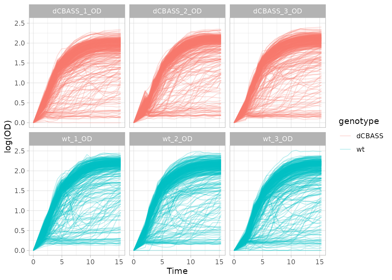
Notice how now the y-axis starts at 0.
Low dimensional representations.
Now that we have pre-processed data we can compute a low-dimensional
representation of our data. DGrowthR offers the possibility
to do this either with a functional PCA, or a UMAP embedding.
dgobj <- estimate_fpca(dgobj)
#> [DGrowthR::estimate_fpca] >> Estimating functional Principal Components
#> [DGrowthR::estimate_fpca] >> Embedding optical density data
#> Warning in CheckData(Ly, Lt): There is a time gap of at least 10% of the
#> observed range across subjects
dgobj <- estimate_umap(dgobj)
#> [DGrowthR::estimate_umap] >> Estimating functional UMAP
#> [DGrowthR::estimate_umap] >> Embedding optical density data
Now we can plot both representations and see what we observe
plot_fpca(dgobj)
plot_umap(dgobj)
plot_fpca(dgobj)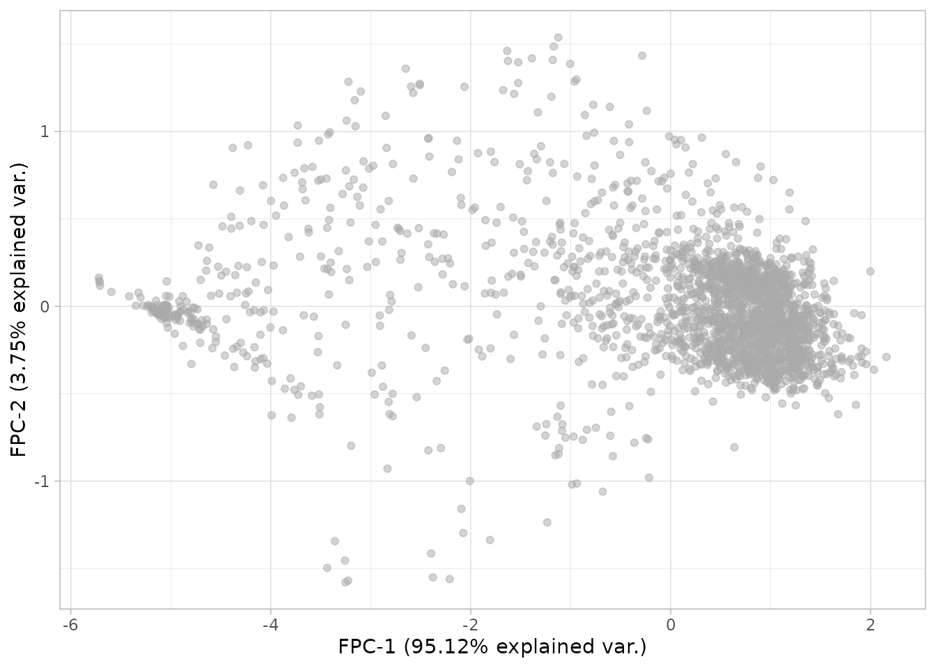
plot_umap(dgobj)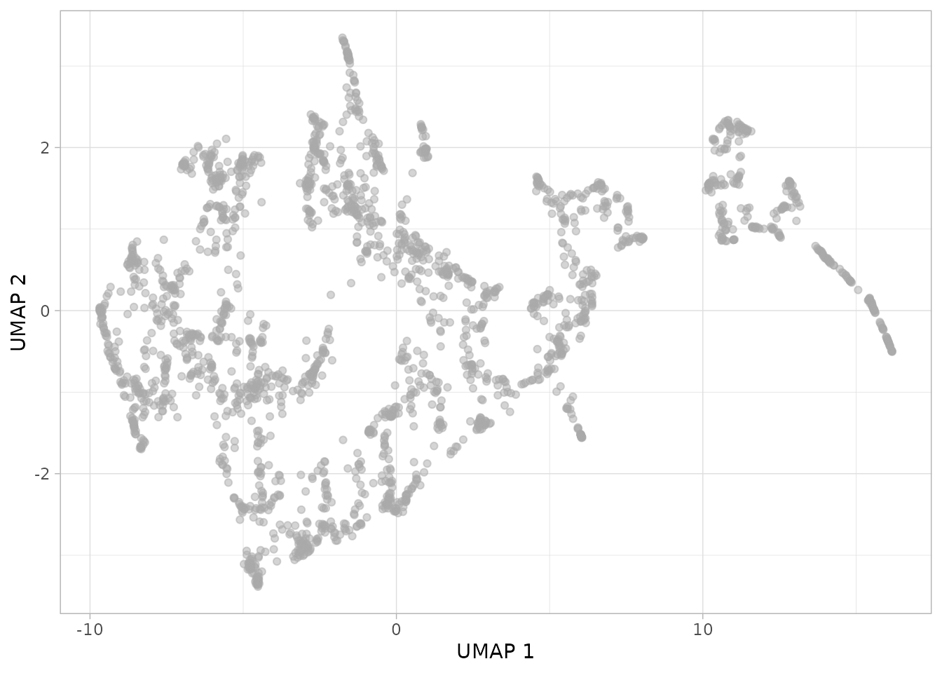
This is looking interesting. One can further investigate what is being captured by coloring a given covariate in the metadata.
plot_umap(dgobj, color = "genotype")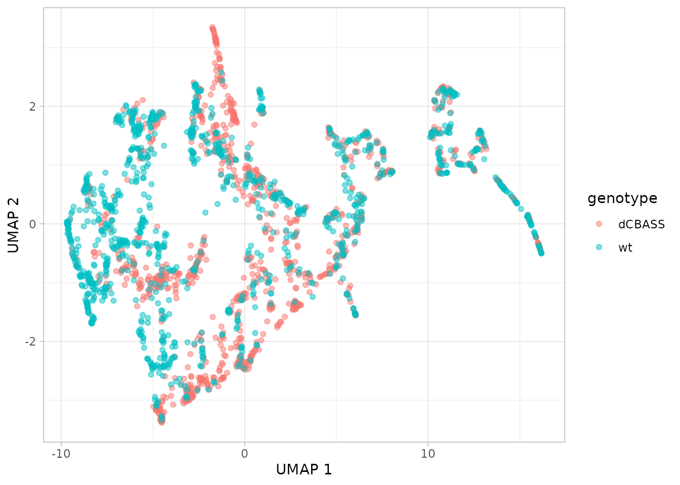
One can also visualize certain growth parameters that are calculated by DGrowthR. That is discussed in the next section.
Clustering.
One can cluster growth curves based on their low-dimensinal embeddings in the fPCA or UMAP. This is acheived by the `
# Clustering based on FPCA coordinates
dgobj <- clustering(dgobj, embedding="fpca")
#> Clustering using fPCA coordinates...
#> [DGrowthR::clustering] >> Density based clustering with DBSCAN
#> [DGrowthR::clustering] >> Using K-nearest neighbors: 23
#> [DGrowthR::clustering] >> Automatic determination of optimal eps...
#> [DGrowthR::clustering] >> Using eps value: 0.258811281594046
#> [DGrowthR::clustering] >> Updating cluster_assignment slot..
#> [DGrowthR::clustering] >> Finished


# Now you can plot cluster assignment
plot_fpca(dgobj, color = "cluster_assignment")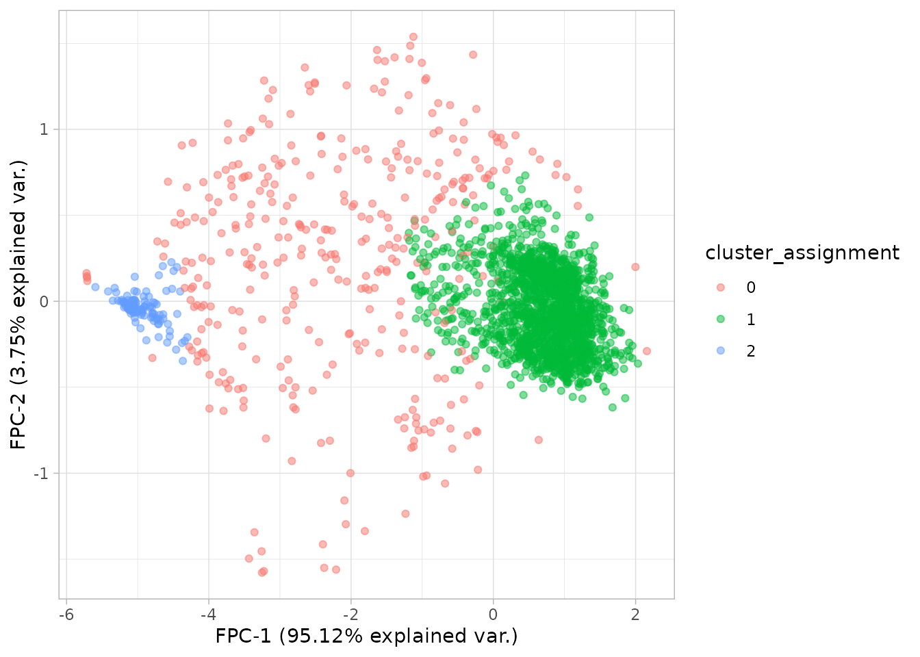
Since we know that we are clustering the individual growth curves, we can plot our growth curves with updated metadata
plot_growth_curves(dgobj, facet="cluster_assignment", color="genotype")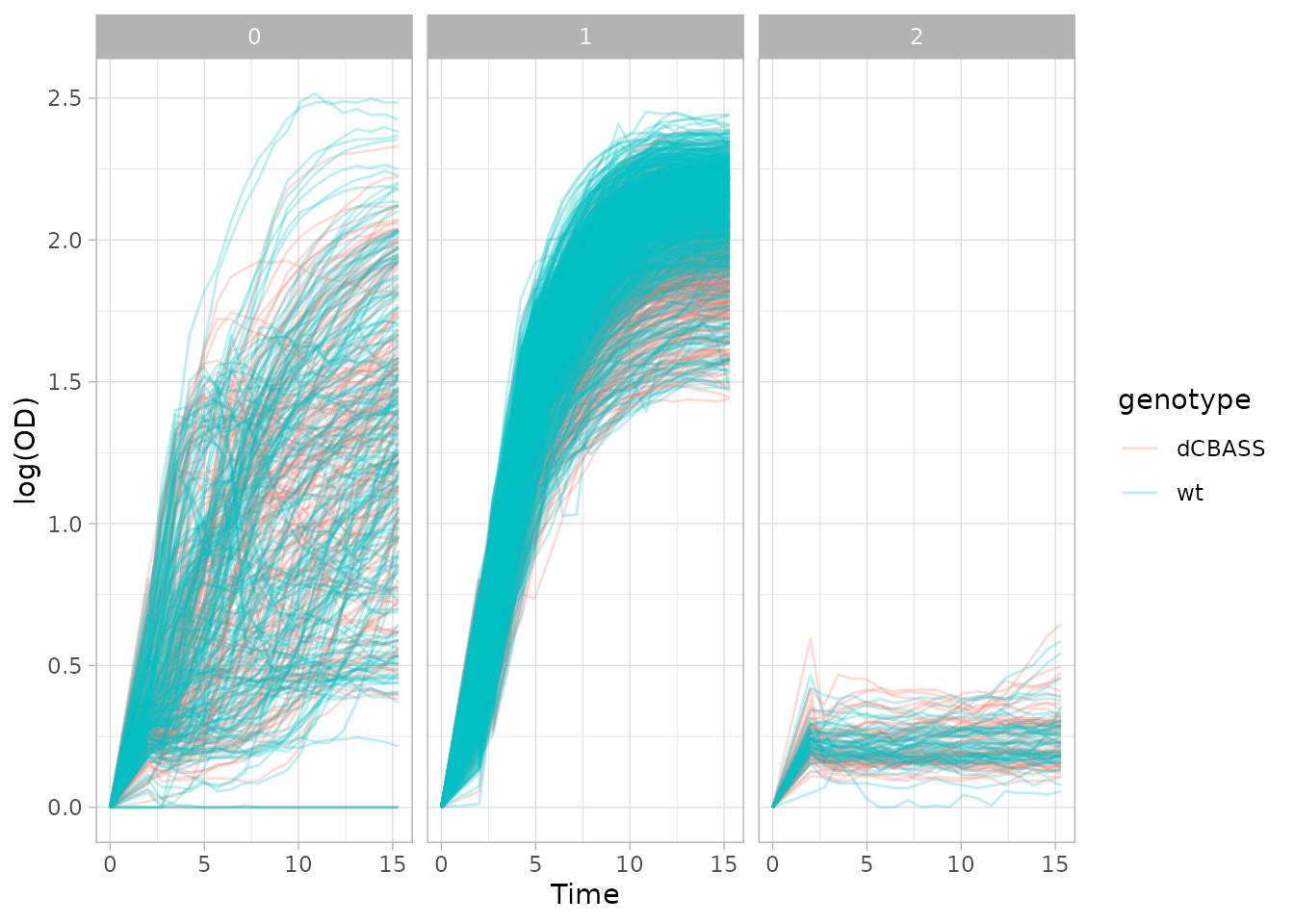
Of course one can play around with clustering by changing the UMAP or fPCA embedding parameters, and also the clustering parameters themselves.
Estimating growth parameters.
Now that we have explored our data a bit, we can get some growth
statistics from our data. In principle, we could do this directly after
pre-processing. One of the main features of DGrowthR is
htat it does not assume a specific functional form our growth curves.
This means that we can flexibly model growth curves that do follow a
typical sigmoidal shape. Briefly, a Gaussian Process (GP) is fit to our
growth data (we use the laGP package
for this), and the main growth statistics are gathered from the mean
posterior.
The growth parameters computed are:
-
max_growth: The maximum growth achieved.
-
max_growth_time: The Time at which
max_growth was reached.
-
AUC: The empirical area under the curve.
-
growth_loss: The maximum decrease of growth after
the moment of maximum growth.
-
max_growth_rate_timepoint: The Time at which the
maximum growth rate is acheived.
-
max_growth_rate: The maximum specific growth
rate.
- doubling_time: Equal to .
-
max_death_rate_timepoint: The Time where the lowest
growth rate is observed.
-
max_death_rate: Maximum rate of death. Properly
speaking it is the lowest growth rate.
- lag_phase_timepoint: The Time where lag phase ends and exponential growth begins. We find this as the maximum of the second derivative before max_growth_rate_timepoint.
-
growth_at_lag_phase: Amount of growth when lag
phase ends.
- stationary_phase_timepoint: The Time where the stationary phase starts. We find this as the minimum of the second derivative after max_growth_rate_timepoint. In a typical growth curve, this would correspond to the beginning of the stationary phase. 13 growth_at_stationary_phase: The amount of growth at stationary_phase_timepoint.
KEEP IN MIND the values reported are in the units that were used during modelling. Since our data was log transformed during pre-processing, all growth parameters are in units of log(OD).
To estimate growth parameters, we can use the
estimate_growth_parameters() function.
dgobj.curve_modelling <- estimate_growth_parameters(dgobj, save_gp_data = TRUE)
#> [DGrowthR::estimate_growth_parameters] >> Fitting GP models and estimating growth parameters...
#> [DGrowthR::estimate_growth_parameters] >> Modelling the curve_id field from metadata. 2304 models will be created.
#> | | | 0% | | | 1% | |= | 1% | |= | 2% | |== | 2% | |== | 3% | |== | 4% | |=== | 4% | |=== | 5% | |==== | 5% | |==== | 6% | |===== | 6% | |===== | 7% | |===== | 8% | |====== | 8% | |====== | 9% | |======= | 9% | |======= | 10% | |======= | 11% | |======== | 11% | |======== | 12% | |========= | 12% | |========= | 13% | |========= | 14% | |========== | 14% | |========== | 15% | |=========== | 15% | |=========== | 16% | |============ | 16% | |============ | 17% | |============ | 18% | |============= | 18% | |============= | 19% | |============== | 19% | |============== | 20% | |============== | 21% | |=============== | 21% | |=============== | 22% | |================ | 22% | |================ | 23% | |================ | 24% | |================= | 24% | |================= | 25% | |================== | 25% | |================== | 26% | |=================== | 26% | |=================== | 27% | |=================== | 28% | |==================== | 28% | |==================== | 29% | |===================== | 29% | |===================== | 30% | |===================== | 31% | |====================== | 31% | |====================== | 32% | |======================= | 32% | |======================= | 33% | |======================= | 34% | |======================== | 34% | |======================== | 35% | |========================= | 35% | |========================= | 36% | |========================== | 36% | |========================== | 37% | |========================== | 38% | |=========================== | 38% | |=========================== | 39% | |============================ | 39% | |============================ | 40% | |============================ | 41% | |============================= | 41% | |============================= | 42% | |============================== | 42% | |============================== | 43% | |============================== | 44% | |=============================== | 44% | |=============================== | 45% | |================================ | 45% | |================================ | 46% | |================================= | 46% | |================================= | 47% | |================================= | 48% | |================================== | 48% | |================================== | 49% | |=================================== | 49% | |=================================== | 50% | |=================================== | 51% | |==================================== | 51% | |==================================== | 52% | |===================================== | 52% | |===================================== | 53% | |===================================== | 54% | |====================================== | 54% | |====================================== | 55% | |======================================= | 55% | |======================================= | 56% | |======================================== | 56% | |======================================== | 57% | |======================================== | 58% | |========================================= | 58% | |========================================= | 59% | |========================================== | 59% | |========================================== | 60% | |========================================== | 61% | |=========================================== | 61% | |=========================================== | 62% | |============================================ | 62% | |============================================ | 63% | |============================================ | 64% | |============================================= | 64% | |============================================= | 65% | |============================================== | 65% | |============================================== | 66% | |=============================================== | 66% | |=============================================== | 67% | |=============================================== | 68% | |================================================ | 68% | |================================================ | 69% | |================================================= | 69% | |================================================= | 70% | |================================================= | 71% | |================================================== | 71% | |================================================== | 72% | |=================================================== | 72% | |=================================================== | 73% | |=================================================== | 74% | |==================================================== | 74% | |==================================================== | 75% | |===================================================== | 75% | |===================================================== | 76% | |====================================================== | 76% | |====================================================== | 77% | |====================================================== | 78% | |======================================================= | 78% | |======================================================= | 79% | |======================================================== | 79% | |======================================================== | 80% | |======================================================== | 81% | |========================================================= | 81% | |========================================================= | 82% | |========================================================== | 82% | |========================================================== | 83% | |========================================================== | 84% | |=========================================================== | 84% | |=========================================================== | 85% | |============================================================ | 85% | |============================================================ | 86% | |============================================================= | 86% | |============================================================= | 87% | |============================================================= | 88% | |============================================================== | 88% | |============================================================== | 89% | |=============================================================== | 89% | |=============================================================== | 90% | |=============================================================== | 91% | |================================================================ | 91% | |================================================================ | 92% | |================================================================= | 92% | |================================================================= | 93% | |================================================================= | 94% | |================================================================== | 94% | |================================================================== | 95% | |=================================================================== | 95% | |=================================================================== | 96% | |==================================================================== | 96% | |==================================================================== | 97% | |==================================================================== | 98% | |===================================================================== | 98% | |===================================================================== | 99% | |======================================================================| 99% | |======================================================================| 100%
#> [DGrowthR::estimate_growth_parameters] >> Updating growth_parameters slot...
#> [DGrowthR::estimate_growth_parameters] >> Updating gpfit_info slot...
#> [DGrowthR::estimate_growth_parameters] >> Finished!By default, the function models and gathers growth parameters for
each individual curve and saves in the @growth_parameters
slot. We can view it here.
dgobj.curve_modelling@growth_parameters %>%
  rmarkdown::paged_table()
As you can see, the gpfit_id field corresponds to the curve_id. We actually update our low-dimensional embeddings with this data now.
# TODO: ADD THIS AS A FUNCTION?

# Gather growth parameters
growth_params <- dgobj.curve_modelling@growth_parameters %>%
  rename("curve_id" = "gpfit_id")

# Add to metadata
dgobj.curve_modelling@metadata <- dgobj.curve_modelling@metadata %>%
  left_join(growth_params, by="curve_id")

# Replot
plot_fpca(dgobj.curve_modelling, color = "AUC")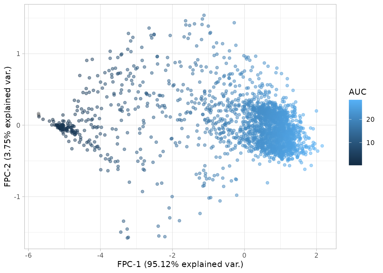
Modelling groups of curves.
One additional advantage of using GP to model our curves is that we can now model several growth curves at the same time! Instead of modelling one curve at a time, we can jointly model all replicate curves that were gathered in the same experimental conditions. For example, in Brenzinger 2024 they analyse the response of a CBASS strain against the wildtype when confronted with different compounds. We can jointly analyse all growth curves coming from the same genotype_compound combination.
dgobj.genotype_well <- estimate_growth_parameters(dgobj,
model_covariate="genotype_well", # covariate in metadata to model
save_gp_data = TRUE, # Save the GP data
n_cores=3)
#> [DGrowthR::estimate_growth_parameters] >> Fitting GP models and estimating growth parameters...
#> [DGrowthR::estimate_growth_parameters] >> Modelling the genotype_well field from metadata. 768 models will be created.
#> | | | 0% | | | 1% | |= | 1% | |= | 2% | |== | 2% | |== | 3% | |== | 4% | |=== | 4% | |=== | 5% | |==== | 5% | |==== | 6% | |===== | 7% | |===== | 8% | |====== | 8% | |====== | 9% | |======= | 9% | |======= | 10% | |======= | 11% | |======== | 11% | |======== | 12% | |========= | 12% | |========= | 13% | |========= | 14% | |========== | 14% | |========== | 15% | |=========== | 15% | |=========== | 16% | |============ | 17% | |============ | 18% | |============= | 18% | |============= | 19% | |============== | 19% | |============== | 20% | |============== | 21% | |=============== | 21% | |=============== | 22% | |================ | 22% | |================ | 23% | |================ | 24% | |================= | 24% | |================= | 25% | |================== | 25% | |================== | 26% | |=================== | 26% | |=================== | 27% | |=================== | 28% | |==================== | 28% | |==================== | 29% | |===================== | 29% | |===================== | 30% | |===================== | 31% | |====================== | 31% | |====================== | 32% | |======================= | 32% | |======================= | 33% | |======================== | 34% | |======================== | 35% | |========================= | 35% | |========================= | 36% | |========================== | 36% | |========================== | 37% | |========================== | 38% | |=========================== | 38% | |=========================== | 39% | |============================ | 39% | |============================ | 40% | |============================ | 41% | |============================= | 41% | |============================= | 42% | |============================== | 42% | |============================== | 43% | |=============================== | 44% | |=============================== | 45% | |================================ | 45% | |================================ | 46% | |================================= | 46% | |================================= | 47% | |================================= | 48% | |================================== | 48% | |================================== | 49% | |=================================== | 49% | |=================================== | 50% | |=================================== | 51% | |==================================== | 51% | |==================================== | 52% | |===================================== | 52% | |===================================== | 53% | |===================================== | 54% | |====================================== | 54% | |====================================== | 55% | |======================================= | 55% | |======================================= | 56% | |======================================== | 57% | |======================================== | 58% | |========================================= | 58% | |========================================= | 59% | |========================================== | 59% | |========================================== | 60% | |========================================== | 61% | |=========================================== | 61% | |=========================================== | 62% | |============================================ | 62% | |============================================ | 63% | |============================================ | 64% | |============================================= | 64% | |============================================= | 65% | |============================================== | 65% | |============================================== | 66% | |=============================================== | 67% | |=============================================== | 68% | |================================================ | 68% | |================================================ | 69% | |================================================= | 69% | |================================================= | 70% | |================================================= | 71% | |================================================== | 71% | |================================================== | 72% | |=================================================== | 72% | |=================================================== | 73% | |=================================================== | 74% | |==================================================== | 74% | |==================================================== | 75% | |===================================================== | 75% | |===================================================== | 76% | |====================================================== | 76% | |====================================================== | 77% | |====================================================== | 78% | |======================================================= | 78% | |======================================================= | 79% | |======================================================== | 79% | |======================================================== | 80% | |======================================================== | 81% | |========================================================= | 81% | |========================================================= | 82% | |========================================================== | 82% | |========================================================== | 83% | |=========================================================== | 84% | |=========================================================== | 85% | |============================================================ | 85% | |============================================================ | 86% | |============================================================= | 86% | |============================================================= | 87% | |============================================================= | 88% | |============================================================== | 88% | |============================================================== | 89% | |=============================================================== | 89% | |=============================================================== | 90% | |=============================================================== | 91% | |================================================================ | 91% | |================================================================ | 92% | |================================================================= | 92% | |================================================================= | 93% | |================================================================== | 94% | |================================================================== | 95% | |=================================================================== | 95% | |=================================================================== | 96% | |==================================================================== | 96% | |==================================================================== | 97% | |==================================================================== | 98% | |===================================================================== | 98% | |===================================================================== | 99% | |======================================================================| 99% | |======================================================================| 100%
#> [DGrowthR::estimate_growth_parameters] >> Updating growth_parameters slot...
#> [DGrowthR::estimate_growth_parameters] >> Updating gpfit_info slot...
#> [DGrowthR::estimate_growth_parameters] >> Finished!Now gpfit_id indicates each group modelled.
dgobj.genotype_well@growth_parameters %>%
  rmarkdown::paged_table()
Additionally, we also indicated that we should save the mean GP
posterior. This can now be accessed in the @gpfit_info
field. We can also now plot this information as below.
plot_gp(dgobj.genotype_well, gpfit_id = "dCBASS_A11", show_input_od=TRUE)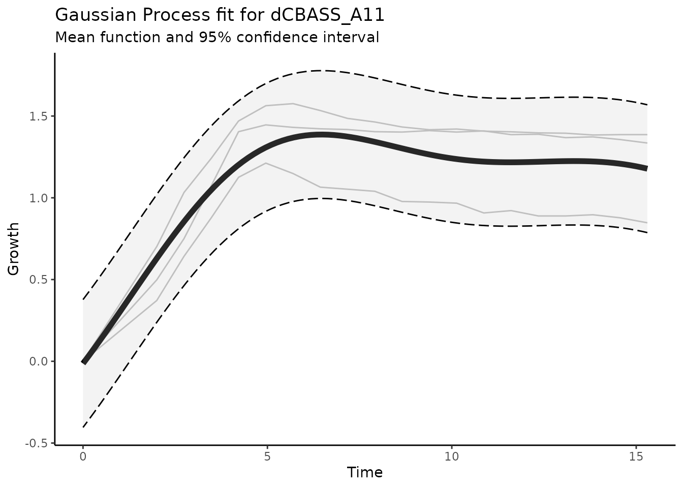
Yet another great trick we can do is sample the posterior of the GP to gather an arbitrary number of synthetic growth curves. We can then gather the growth statistics from these sampled curves and get the mean and standard deviation of the growth parameters.
Keep in mind that it only makes sense to do this when the modeled covariate contains more than one growth curve per group.
dgobj.genotype_well.posterior <- estimate_growth_parameters(dgobj,
                                                  model_covariate="genotype_well",

                                                  predict_n_steps = 100, # Predict a lower number of GP points to speed up

                                                  sample_posterior_gpfit=TRUE, # Sample the posterior to get mean and sd of each parameter

                                                  sample_n_curves=10,  # Number of curves to sample from posterior. 10 for speed.
                                                  save_gp_data = FALSE,
                                                  n_cores=4) # Increased number of cores
Now we can see that our growth statistics have a mean and standard deviation.
dgobj.genotype_well.posterior@growth_parameters %>%
  rmarkdown::paged_table()
Polyauxic growth.
In many research applications, it is important to detect and characterize polyauxic growth. Polyauxic growth is a phenomenon where multiple distinct growth phases are observed in a single growth curve. This can be indicative of complex underlying biological processes, such as diauxic shifts, where an organism switches from one energy source to another, or the presence of subpopulations with different growth dynamics.
In DGrowthR we can detect polyauxic growth when
modelling growth curves with the
estimate_growth_parameters() function. To do this, we can
set the detect_polyauxic parameter to TRUE. This will
trigger an additional step in the growth parameter estimation process
where the function will look for multiple growth phases in the mean
posterior of the GP fit. The detection of polyauxic growth is based on
two criteria:
1. polyauxic_ratio_threshold: This is the minimum ratio
between the maximum growth of the second growth phase and the maximum
growth of the first growth phase. For example, if this is set to 0.5,
the second growth phase must have a maximum growth that is at least 50%
of the maximum growth of the first phase to be considered a valid
polyauxic phase.
2. polyauxic_parameter_criteria: This is the growth
parameter that is used to determine the maximum growth of each phase. By
default, this is set to “carrying_capacity”, which means that the
maximum growth of each phase is determined by the carrying capacity of
that phase. However, other parameters such as “growth_rate” could also
be used.
dgobj.polyauxic <- estimate_growth_parameters(dgobj,
model_covariate="genotype_well", # covariate in metadata to model
save_gp_data = TRUE, # Save the GP data
n_cores=3,
# Polyauxic detection
detect_polyauxic = TRUE, # Detect polyauxic growth
polyauxic_ratio_threshold = 0.5,
polyauxic_parameter_criteria = "carrying_capacity")
#> [DGrowthR::estimate_growth_parameters] >> Fitting GP models and estimating growth parameters...
#> [DGrowthR::estimate_growth_parameters] >> Modelling the genotype_well field from metadata. 768 models will be created.
#> | | | 0% | | | 1% | |= | 1% | |= | 2% | |== | 2% | |== | 3% | |== | 4% | |=== | 4% | |=== | 5% | |==== | 5% | |==== | 6% | |===== | 7% | |===== | 8% | |====== | 8% | |====== | 9% | |======= | 9% | |======= | 10% | |======= | 11% | |======== | 11% | |======== | 12% | |========= | 12% | |========= | 13% | |========= | 14% | |========== | 14% | |========== | 15% | |=========== | 15% | |=========== | 16% | |============ | 17% | |============ | 18% | |============= | 18% | |============= | 19% | |============== | 19% | |============== | 20% | |============== | 21% | |=============== | 21% | |=============== | 22% | |================ | 22% | |================ | 23% | |================ | 24% | |================= | 24% | |================= | 25% | |================== | 25% | |================== | 26% | |=================== | 26% | |=================== | 27% | |=================== | 28% | |==================== | 28% | |==================== | 29% | |===================== | 29% | |===================== | 30% | |===================== | 31% | |====================== | 31% | |====================== | 32% | |======================= | 32% | |======================= | 33% | |======================== | 34% | |======================== | 35% | |========================= | 35% | |========================= | 36% | |========================== | 36% | |========================== | 37% | |========================== | 38% | |=========================== | 38% | |=========================== | 39% | |============================ | 39% | |============================ | 40% | |============================ | 41% | |============================= | 41% | |============================= | 42% | |============================== | 42% | |============================== | 43% | |=============================== | 44% | |=============================== | 45% | |================================ | 45% | |================================ | 46% | |================================= | 46% | |================================= | 47% | |================================= | 48% | |================================== | 48% | |================================== | 49% | |=================================== | 49% | |=================================== | 50% | |=================================== | 51% | |==================================== | 51% | |==================================== | 52% | |===================================== | 52% | |===================================== | 53% | |===================================== | 54% | |====================================== | 54% | |====================================== | 55% | |======================================= | 55% | |======================================= | 56% | |======================================== | 57% | |======================================== | 58% | |========================================= | 58% | |========================================= | 59% | |========================================== | 59% | |========================================== | 60% | |========================================== | 61% | |=========================================== | 61% | |=========================================== | 62% | |============================================ | 62% | |============================================ | 63% | |============================================ | 64% | |============================================= | 64% | |============================================= | 65% | |============================================== | 65% | |============================================== | 66% | |=============================================== | 67% | |=============================================== | 68% | |================================================ | 68% | |================================================ | 69% | |================================================= | 69% | |================================================= | 70% | |================================================= | 71% | |================================================== | 71% | |================================================== | 72% | |=================================================== | 72% | |=================================================== | 73% | |=================================================== | 74% | |==================================================== | 74% | |==================================================== | 75% | |===================================================== | 75% | |===================================================== | 76% | |====================================================== | 76% | |====================================================== | 77% | |====================================================== | 78% | |======================================================= | 78% | |======================================================= | 79% | |======================================================== | 79% | |======================================================== | 80% | |======================================================== | 81% | |========================================================= | 81% | |========================================================= | 82% | |========================================================== | 82% | |========================================================== | 83% | |=========================================================== | 84% | |=========================================================== | 85% | |============================================================ | 85% | |============================================================ | 86% | |============================================================= | 86% | |============================================================= | 87% | |============================================================= | 88% | |============================================================== | 88% | |============================================================== | 89% | |=============================================================== | 89% | |=============================================================== | 90% | |=============================================================== | 91% | |================================================================ | 91% | |================================================================ | 92% | |================================================================= | 92% | |================================================================= | 93% | |================================================================== | 94% | |================================================================== | 95% | |=================================================================== | 95% | |=================================================================== | 96% | |==================================================================== | 96% | |==================================================================== | 97% | |==================================================================== | 98% | |===================================================================== | 98% | |===================================================================== | 99% | |======================================================================| 99% | |======================================================================| 100%
#> [DGrowthR::estimate_growth_parameters] >> Updating growth_parameters slot...
#> [DGrowthR::estimate_growth_parameters] >> Updating gpfit_info slot...
#> [DGrowthR::estimate_growth_parameters] >> Finished!The results can be viewed in the @growth_parameters
slot. The number of growth phases detected is indicated in the
n_growth_phases field, and the maximum growth of each
phase is indicated in the max_growth_phase_1,
max_growth_phase_2, etc. fields. Below we can see all
of the growth curves where more than one growth phase was detected and
where at least 0.2 of the maximum oeverall growth.
dgobj.polyauxic@growth_parameters %>%
  filter(n_growth_phases > 1,
         max_growth > 0.2) %>%
  rmarkdown::paged_table()
Below we plot an example curve with two growth phases. The vertical lines indicate the transition between different growth phases.
plot_gp(dgobj.polyauxic, gpfit_id = "wt_A10", show_input_od=TRUE) +
  geom_vline(xintercept = c(0, 8.037414, 14.99287))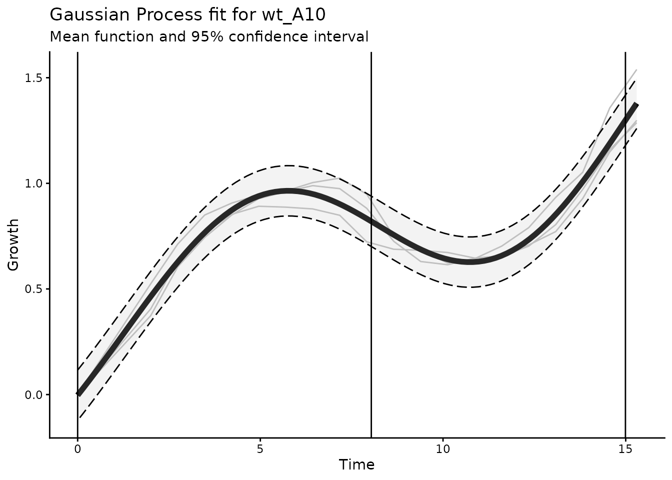
Differential growth.
One of the other main features of DGrowthR is the
ability to compare growth curves gathered from different experimental
conditions. This done via a likelihood ratio test. Briefly, two GP
models are fit: a null model where all growth curves are modeled
jointly, and an alternative model where an additional covariate is added
to the design matrix indicating whether the growth curve come from the
reference or treatment condition. Then the log-likelihood of these two
models is compared, giving us the likelihood ratio test statistic.
In DgrowthR all of these steps can be run with the
growth_comparison() function. Here a comparison is
indicated to the comparison_info parameter as a vector
consisting of (metatada_field, treatment_value, reference_value). The
metadata field should be a field in the metadata, and the treatment and
reference values should be found in said field. These groups of growth
curves are compared to eachother as described above.
Following our example, we can compare how genotype affects the response to the same compound.
object.comparison <- growth_comparison(object = dgobj,

                                       # A comparison is indicated as metadata_field, treatment, reference.
                                       comparison_info = c("genotype_well", "dCBASS_O1" ,"wt_O1"),
                                       save_gp_data = TRUE)
#> [DGrowthR::growth_comparison] >> Comparing dCBASS_O1 to wt_O1 from the genotype_well field.
#> [DGrowthR::growth_comparison] >> Finished!


# View result of comparison
growth_comparison_result(object.comparison) %>%
  rmarkdown::paged_table()
Here we see the result of our comparison.
-
likelihood_ratio: Indicates the test statistic for
the likelihood ratio test. It is equal to
llik.alternative_model -
llik.null_model.
-
llik.alternative_model: The log-likelihood of the
GP fit with the alternative model.
-
llik.null_model: The log-likelihood of the GP fit
with the null model.
-
AUC.treatment: The AUC of the alternative model fit
for the treatment growth curves.
- AUC.reference: The AUC of the alternative model fit for the reference growth curves.
-
AUC.FoldChange: Equal to
.
-
max_growth.treatment: Maximum growth determined for
the alternative model fit for the treatment growth curves.
-
max_growth.reference: Maximum growth determined for
the alternative model fit for the reference growth curves.
-
max_growth.FoldChange: Equal to
.
- euclidean.distance: The euclidean distance between the model fit for the treatment and alternative curves.
We can get a better intuition by looking at a visual representation of our model. Below we see the fit of the null model, where all growth curves are modelled jointly, independent of the genotype. We can clearly see that the fit is poor.
model_plots <- plot_growth_comparison(object.comparison)

model_plots$null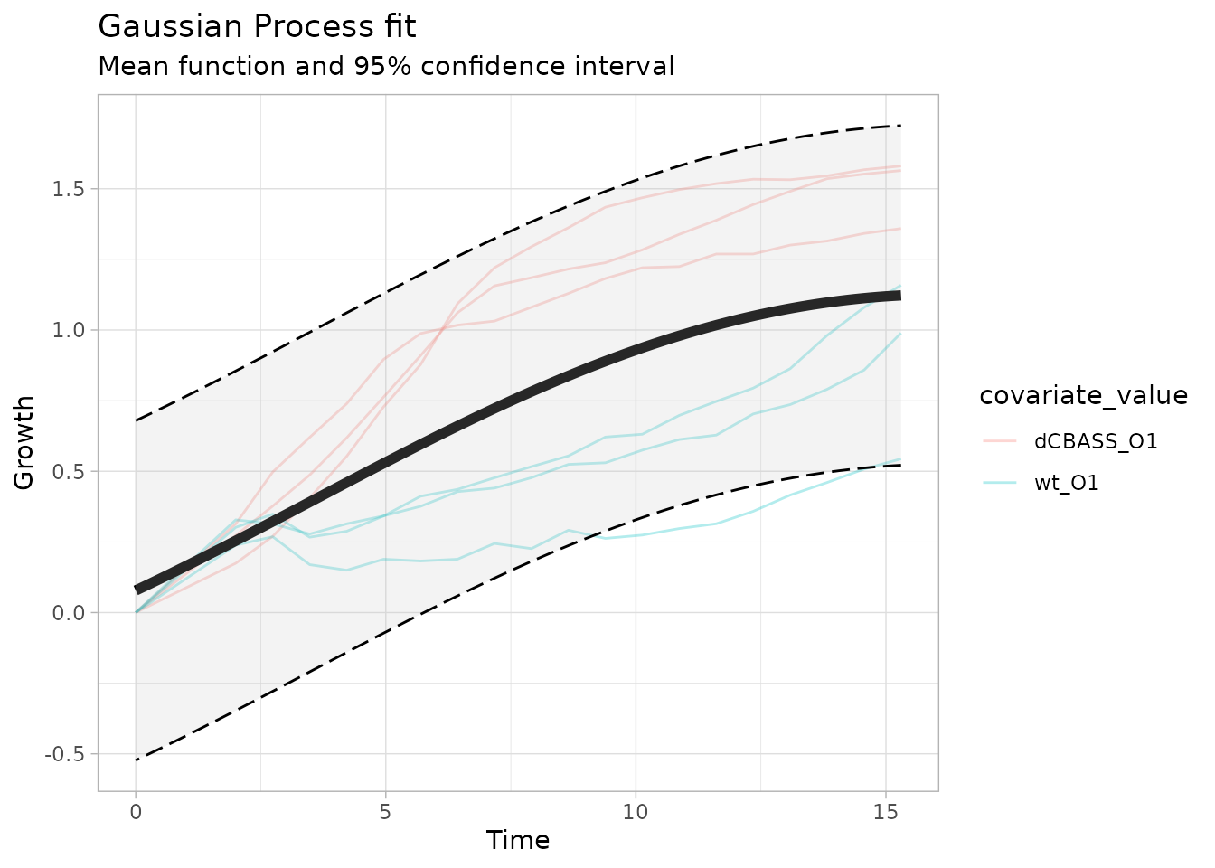
The alternative model fits the original growth curves much better, indicating that these two groups might be significantly different.
model_plots$alternative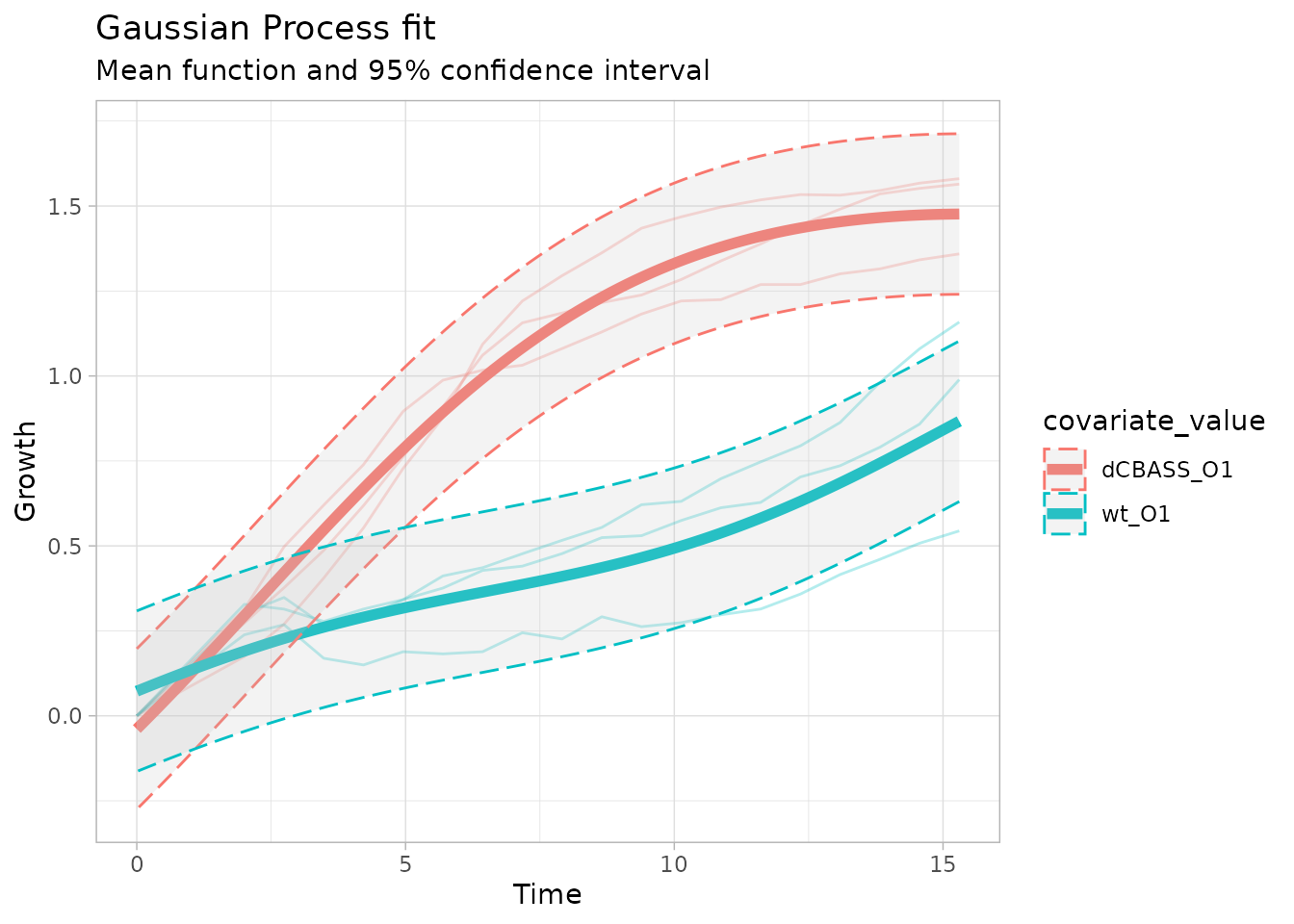
Of course, up until this point we only have visual evidence for this
significant difference. We can get some statistical significance by
performing a permutation test. In DGrowthR the permutation
test consists of randomly shuffling the label of each growth curve and
computing the log-likelihood of the alternative GP model when these
curves are shuffled. Doing this several times can give us an idea of the
the distribution of the likelihood ratio test statistic when curves are
randomly assigned. In this case we can set the
permutation_test parameter and indicate the number of
permutations we would like to perform.
object.comparison.permutation <- growth_comparison(object = dgobj,
comparison_info = c("genotype_well", "dCBASS_O1" ,"wt_O1"),
permutation_test=TRUE,
n_permutations = 100, # Here we use 100 for speed but should probably be more
n_cores = 1,
save_gp_data = FALSE)
#> [DGrowthR::growth_comparison] >> Comparing dCBASS_O1 to wt_O1 from the genotype_well field.
#> [DGrowthR::perm_test] >> Perform permutation test with 100 permutations
#> | | | 0% | |= | 1% | |= | 2% | |== | 3% | |=== | 4% | |==== | 5% | |==== | 6% | |===== | 7% | |====== | 8% | |====== | 9% | |======= | 10% | |======== | 11% | |======== | 12% | |========= | 13% | |========== | 14% | |========== | 15% | |=========== | 16% | |============ | 17% | |============= | 18% | |============= | 19% | |============== | 20% | |=============== | 21% | |=============== | 22% | |================ | 23% | |================= | 24% | |================== | 25% | |================== | 26% | |=================== | 27% | |==================== | 28% | |==================== | 29% | |===================== | 30% | |====================== | 31% | |====================== | 32% | |======================= | 33% | |======================== | 34% | |======================== | 35% | |========================= | 36% | |========================== | 37% | |=========================== | 38% | |=========================== | 39% | |============================ | 40% | |============================= | 41% | |============================= | 42% | |============================== | 43% | |=============================== | 44% | |================================ | 45% | |================================ | 46% | |================================= | 47% | |================================== | 48% | |================================== | 49% | |=================================== | 50% | |==================================== | 51% | |==================================== | 52% | |===================================== | 53% | |====================================== | 54% | |====================================== | 55% | |======================================= | 56% | |======================================== | 57% | |========================================= | 58% | |========================================= | 59% | |========================================== | 60% | |=========================================== | 61% | |=========================================== | 62% | |============================================ | 63% | |============================================= | 64% | |============================================== | 65% | |============================================== | 66% | |=============================================== | 67% | |================================================ | 68% | |================================================ | 69% | |================================================= | 70% | |================================================== | 71% | |================================================== | 72% | |=================================================== | 73% | |==================================================== | 74% | |==================================================== | 75% | |===================================================== | 76% | |====================================================== | 77% | |======================================================= | 78% | |======================================================= | 79% | |======================================================== | 80% | |========================================================= | 81% | |========================================================= | 82% | |========================================================== | 83% | |=========================================================== | 84% | |============================================================ | 85% | |============================================================ | 86% | |============================================================= | 87% | |============================================================== | 88% | |============================================================== | 89% | |=============================================================== | 90% | |================================================================ | 91% | |================================================================ | 92% | |================================================================= | 93% | |================================================================== | 94% | |================================================================== | 95% | |=================================================================== | 96% | |==================================================================== | 97% | |===================================================================== | 98% | |===================================================================== | 99% | |======================================================================| 100%
#> [DGrowthR::perm_test] >> Time taken to perform permutation test: 5 second(s)
#> [DGrowthR::growth_comparison] >> Finished!As we can see below, a new field is added to the results empirical_p.value. This empirical p-value is calculated as the fraction of premuted test statistics that are larger than the observed test statistic. We can see below that the empirical_p.value is 0.009, which is quite good considering this is the lowest possible p-value in our setup.
growth_comparison_result(object.comparison.permutation)
#>                            comparison likelihood_ratio llik.alternative_model
#> 1 genotype_well: dCBASS_O1 v.s. wt_O1         107.5764              -18.80289
#>   llik.null_model AUC.treatment AUC.reference AUC.FoldChange
#> 1       -126.3793      14.97957      6.555202       2.285142
#>   max_growth.treatment max_growth.reference max_growth.FoldChange
#> 1             1.476493            0.8666307              1.703716
#>   euclidean.distance empirical_p.value
#> 1           6.224746         0.1188119
We can get a visual inspection of the null vs observed test statistic below
plot_likelihood_ratio(object.comparison.permutation, num_bins = 50)
#> Warning: Using `size` aesthetic for lines was deprecated in ggplot2 3.4.0.
#> ℹ Please use `linewidth` instead.
#> ℹ The deprecated feature was likely used in the DGrowthR package.
#>   Please report the issue at
#>   <https://github.com/bio-datascience/DGrowthR/issues>.
#> This warning is displayed once per session.
#> Call `lifecycle::last_lifecycle_warnings()` to see where this warning was
#> generated.
#> Ignoring unknown labels:
#> • colour : "Line Type"
#> • linetype : "Line Type"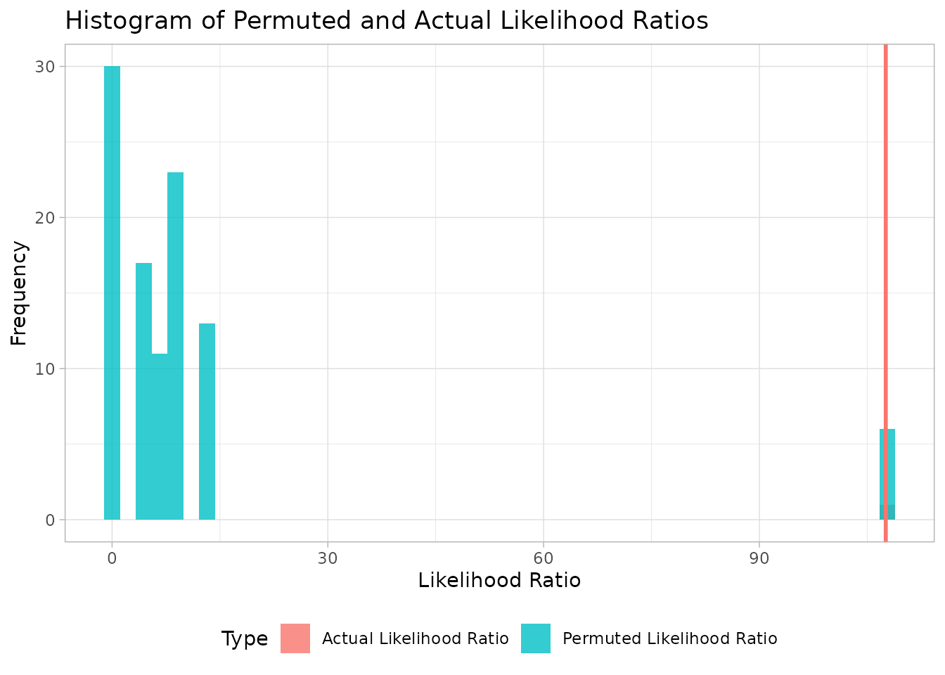
We can also plot the difference between the reference and treatment condition over time
plot_od_difference(object.comparison)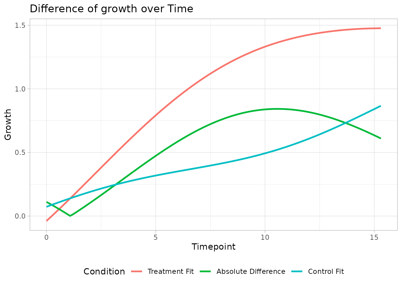
Multiple comparisons.
Now let’s imagine that we actually want to make several comparisons in one go. For that we can use the multiple_comparisons function. It is actually quite similar to the function above only that now we provide a list that contains all of the comparisons we want to make
contrast_list <- list(c("genotype_well", "dCBASS_O1" ,"wt_O1"),
c("genotype_well", "dCBASS_A1" ,"wt_A1"),
c("genotype_well", "dCBASS_B1" ,"wt_B1"))
# Returns a dataframe
result_list <- multiple_comparisons(dgobj,contrast_list,
permutation_test = TRUE,
n_permutations = 100,
save_perm_stats = TRUE) # This is important to make use of the gamma-approximated p-values
#> [DGrowthR::multiple_comparisons] >> Computing genotype_well: dCBASS_O1 vs wt_O1 at step 1 of 3
#> [DGrowthR::growth_comparison] >> Comparing dCBASS_O1 to wt_O1 from the genotype_well field.
#> [DGrowthR::perm_test] >> Perform permutation test with 100 permutations
#> | | | 0% | |= | 1% | |= | 2% | |== | 3% | |=== | 4% | |==== | 5% | |==== | 6% | |===== | 7% | |====== | 8% | |====== | 9% | |======= | 10% | |======== | 11% | |======== | 12% | |========= | 13% | |========== | 14% | |========== | 15% | |=========== | 16% | |============ | 17% | |============= | 18% | |============= | 19% | |============== | 20% | |=============== | 21% | |=============== | 22% | |================ | 23% | |================= | 24% | |================== | 25% | |================== | 26% | |=================== | 27% | |==================== | 28% | |==================== | 29% | |===================== | 30% | |====================== | 31% | |====================== | 32% | |======================= | 33% | |======================== | 34% | |======================== | 35% | |========================= | 36% | |========================== | 37% | |=========================== | 38% | |=========================== | 39% | |============================ | 40% | |============================= | 41% | |============================= | 42% | |============================== | 43% | |=============================== | 44% | |================================ | 45% | |================================ | 46% | |================================= | 47% | |================================== | 48% | |================================== | 49% | |=================================== | 50% | |==================================== | 51% | |==================================== | 52% | |===================================== | 53% | |====================================== | 54% | |====================================== | 55% | |======================================= | 56% | |======================================== | 57% | |========================================= | 58% | |========================================= | 59% | |========================================== | 60% | |=========================================== | 61% | |=========================================== | 62% | |============================================ | 63% | |============================================= | 64% | |============================================== | 65% | |============================================== | 66% | |=============================================== | 67% | |================================================ | 68% | |================================================ | 69% | |================================================= | 70% | |================================================== | 71% | |================================================== | 72% | |=================================================== | 73% | |==================================================== | 74% | |==================================================== | 75% | |===================================================== | 76% | |====================================================== | 77% | |======================================================= | 78% | |======================================================= | 79% | |======================================================== | 80% | |========================================================= | 81% | |========================================================= | 82% | |========================================================== | 83% | |=========================================================== | 84% | |============================================================ | 85% | |============================================================ | 86% | |============================================================= | 87% | |============================================================== | 88% | |============================================================== | 89% | |=============================================================== | 90% | |================================================================ | 91% | |================================================================ | 92% | |================================================================= | 93% | |================================================================== | 94% | |================================================================== | 95% | |=================================================================== | 96% | |==================================================================== | 97% | |===================================================================== | 98% | |===================================================================== | 99% | |======================================================================| 100%
#> [DGrowthR::perm_test] >> Time taken to perform permutation test: 5 second(s)
#> [DGrowthR::growth_comparison] >> Finished!
#> [DGrowthR::multiple_comparisons] >> Computing genotype_well: dCBASS_A1 vs wt_A1 at step 2 of 3
#> [DGrowthR::growth_comparison] >> Comparing dCBASS_A1 to wt_A1 from the genotype_well field.
#> [DGrowthR::perm_test] >> Perform permutation test with 100 permutations
#> | | | 0% | |= | 1% | |= | 2% | |== | 3% | |=== | 4% | |==== | 5% | |==== | 6% | |===== | 7% | |====== | 8% | |====== | 9% | |======= | 10% | |======== | 11% | |======== | 12% | |========= | 13% | |========== | 14% | |========== | 15% | |=========== | 16% | |============ | 17% | |============= | 18% | |============= | 19% | |============== | 20% | |=============== | 21% | |=============== | 22% | |================ | 23% | |================= | 24% | |================== | 25% | |================== | 26% | |=================== | 27% | |==================== | 28% | |==================== | 29% | |===================== | 30% | |====================== | 31% | |====================== | 32% | |======================= | 33% | |======================== | 34% | |======================== | 35% | |========================= | 36% | |========================== | 37% | |=========================== | 38% | |=========================== | 39% | |============================ | 40% | |============================= | 41% | |============================= | 42% | |============================== | 43% | |=============================== | 44% | |================================ | 45% | |================================ | 46% | |================================= | 47% | |================================== | 48% | |================================== | 49% | |=================================== | 50% | |==================================== | 51% | |==================================== | 52% | |===================================== | 53% | |====================================== | 54% | |====================================== | 55% | |======================================= | 56% | |======================================== | 57% | |========================================= | 58% | |========================================= | 59% | |========================================== | 60% | |=========================================== | 61% | |=========================================== | 62% | |============================================ | 63% | |============================================= | 64% | |============================================== | 65% | |============================================== | 66% | |=============================================== | 67% | |================================================ | 68% | |================================================ | 69% | |================================================= | 70% | |================================================== | 71% | |================================================== | 72% | |=================================================== | 73% | |==================================================== | 74% | |==================================================== | 75% | |===================================================== | 76% | |====================================================== | 77% | |======================================================= | 78% | |======================================================= | 79% | |======================================================== | 80% | |========================================================= | 81% | |========================================================= | 82% | |========================================================== | 83% | |=========================================================== | 84% | |============================================================ | 85% | |============================================================ | 86% | |============================================================= | 87% | |============================================================== | 88% | |============================================================== | 89% | |=============================================================== | 90% | |================================================================ | 91% | |================================================================ | 92% | |================================================================= | 93% | |================================================================== | 94% | |================================================================== | 95% | |=================================================================== | 96% | |==================================================================== | 97% | |===================================================================== | 98% | |===================================================================== | 99% | |======================================================================| 100%
#> [DGrowthR::perm_test] >> Time taken to perform permutation test: 6 second(s)
#> [DGrowthR::growth_comparison] >> Finished!
#> [DGrowthR::multiple_comparisons] >> Computing genotype_well: dCBASS_B1 vs wt_B1 at step 3 of 3
#> [DGrowthR::growth_comparison] >> Comparing dCBASS_B1 to wt_B1 from the genotype_well field.
#> [DGrowthR::perm_test] >> Perform permutation test with 100 permutations
#> | | | 0% | |= | 1% | |= | 2% | |== | 3% | |=== | 4% | |==== | 5% | |==== | 6% | |===== | 7% | |====== | 8% | |====== | 9% | |======= | 10% | |======== | 11% | |======== | 12% | |========= | 13% | |========== | 14% | |========== | 15% | |=========== | 16% | |============ | 17% | |============= | 18% | |============= | 19% | |============== | 20% | |=============== | 21% | |=============== | 22% | |================ | 23% | |================= | 24% | |================== | 25% | |================== | 26% | |=================== | 27% | |==================== | 28% | |==================== | 29% | |===================== | 30% | |====================== | 31% | |====================== | 32% | |======================= | 33% | |======================== | 34% | |======================== | 35% | |========================= | 36% | |========================== | 37% | |=========================== | 38% | |=========================== | 39% | |============================ | 40% | |============================= | 41% | |============================= | 42% | |============================== | 43% | |=============================== | 44% | |================================ | 45% | |================================ | 46% | |================================= | 47% | |================================== | 48% | |================================== | 49% | |=================================== | 50% | |==================================== | 51% | |==================================== | 52% | |===================================== | 53% | |====================================== | 54% | |====================================== | 55% | |======================================= | 56% | |======================================== | 57% | |========================================= | 58% | |========================================= | 59% | |========================================== | 60% | |=========================================== | 61% | |=========================================== | 62% | |============================================ | 63% | |============================================= | 64% | |============================================== | 65% | |============================================== | 66% | |=============================================== | 67% | |================================================ | 68% | |================================================ | 69% | |================================================= | 70% | |================================================== | 71% | |================================================== | 72% | |=================================================== | 73% | |==================================================== | 74% | |==================================================== | 75% | |===================================================== | 76% | |====================================================== | 77% | |======================================================= | 78% | |======================================================= | 79% | |======================================================== | 80% | |========================================================= | 81% | |========================================================= | 82% | |========================================================== | 83% | |=========================================================== | 84% | |============================================================ | 85% | |============================================================ | 86% | |============================================================= | 87% | |============================================================== | 88% | |============================================================== | 89% | |=============================================================== | 90% | |================================================================ | 91% | |================================================================ | 92% | |================================================================= | 93% | |================================================================== | 94% | |================================================================== | 95% | |=================================================================== | 96% | |==================================================================== | 97% | |===================================================================== | 98% | |===================================================================== | 99% | |======================================================================| 100%
#> [DGrowthR::perm_test] >> Time taken to perform permutation test: 6 second(s)
#> [DGrowthR::growth_comparison] >> Finished!Now we can view the results in one data.frame as shown below. There is also now an pvalue.adjust field which performs BH correction to the empirical_p.value field after all tests are done.
result_list$result_df %>%
  rmarkdown::paged_table()
Additionally, you can obtain gamma-approximated p-values.
gamma_pvalues(result_list) %>%
  rmarkdown::paged_table()
#> Fitting Gamma (tail > 0) for 2 tests (sequential) ...
#> Done.
That should be good to get you started!